Understanding Spatial Data
Spatial data involves a combination of information about locations and geometric features related that best describe the location. The most commonly used formats to store spatial information are Raster and Vector. A Raster format is a type of digital image represented by grids which can be reduced and enlarged. They are made up of a matrix of pixels with each pixel representing an area within the spatial object. A Vector format consists of geometric shapes organized in the form of shapefiles. A shapefile consist of three files under the extensions .shp, .shx and .dbf which contain the features, indices of shapes and attributes respectively.
Plotting Raster Data
We shall use the getData function in the dismo package to obtain altitude data of Australia and plot them.
aust <- getData('alt', country='Australia', mask=TRUE)## NOTE: rgdal::checkCRSArgs: no proj_defs.dat in PROJ.4 shared files
## NOTE: rgdal::checkCRSArgs: no proj_defs.dat in PROJ.4 shared filesplot(aust)## NOTE: rgdal::checkCRSArgs: no proj_defs.dat in PROJ.4 shared files
## NOTE: rgdal::checkCRSArgs: no proj_defs.dat in PROJ.4 shared files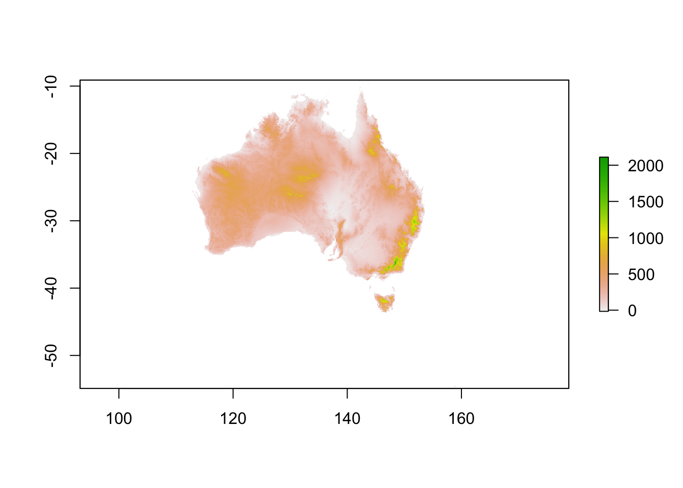
Plotting Shapefiles
Let us visualize the streets and places of Singapore. We can obtain the data from data.gov.sg . We shall project it on top of a base map obtained from OpenStreetMap.
shpfile <- readOGR(dsn='data/street-and-places/', 'StreetsandPlaces')## OGR data source with driver: ESRI Shapefile
## Source: "data/street-and-places/", layer: "StreetsandPlaces"
## with 369 features
## It has 18 fields## NOTE: rgdal::checkCRSArgs: no proj_defs.dat in PROJ.4 shared fileshead(coordinates(shpfile), 5)## coords.x1 coords.x2
## [1,] 28640.40 29320.77
## [2,] 29429.83 28548.69
## [3,] 29224.01 28360.38
## [4,] 29827.20 29664.26
## [5,] 28451.00 29451.78It is observed that the projection system is different than the base map. So we shall transform the projection in to Web Mercator.
crsobj <- CRS("+proj=longlat +datum=WGS84") # Web Mercator projection system## NOTE: rgdal::checkCRSArgs: no proj_defs.dat in PROJ.4 shared filesshpfile.t <- spTransform(shpfile, crsobj) # Applying projection transformation## NOTE: rgdal::checkCRSArgs: no proj_defs.dat in PROJ.4 shared files
## NOTE: rgdal::checkCRSArgs: no proj_defs.dat in PROJ.4 shared filesdf <- as.data.frame(coordinates(shpfile.t)) # Converting to a data frame
df$Name <- shpfile$NAME # Adding names of the location
df$Longitude <- df$coords.x1
df$Latitude <- df$coords.x2
df$coords.x1 <- NULL
df$coords.x2 <- NULL
head(df, 5)## Name Longitude Latitude
## 1 Outram Road 103.8391 1.281441
## 2 Parsi Road 103.8462 1.274459
## 3 Keppel Road 103.8443 1.272756
## 4 Philip Street 103.8497 1.284547
## 5 Pearl's Hill Prison 103.8374 1.282626Now it looks fine to be projected on top of the base map.
sgmap <- get_map(location="Singapore", zoom=11,
                 maptype="roadmap", source="google") # Using Osm base map of Singapore
## Source : https://maps.googleapis.com/maps/api/staticmap?center=Singapore&zoom=11&size=640x640&scale=2&maptype=roadmap&language=en-EN## Source : https://maps.googleapis.com/maps/api/geocode/json?address=Singaporeggmap(sgmap) +
geom_point(data=df,
aes(x=Longitude, y=Latitude),
color='orange', size=1)